The failure that teaches you the most about a temporal knowledge graph doesn't look like one. The system returns an answer that's confident, well-formed, and sourced from a real fact that lives in the graph. It's also wrong, because the fact stopped being true four months ago, and the query that retrieved it never asked about time. When the world changed, the edge was marked invalid and left in place, exactly as the design intends. Then a query that filtered on relationship type but not on validity walked straight past the invalidation and handed the stale edge to an agent that had no way to know it was holding history.
That failure is the gap between a temporal knowledge graph that works in a demo and one that works in production. The demo proves the model can represent time. Production is the year you spend learning that representing time and querying time correctly are two separate disciplines, that the second one isn't automatic, and that every shortcut you take at ingestion or in your indexes comes back as a silently wrong answer months later. Essay 02 covered what bi-temporal modeling means and why it matters. This one covers what it costs to run, the schema choices that lock you in before you understand them, and the query shapes that look fine at a thousand edges and fall over at ten million.
The middle layer is Graphiti, the open-source temporal-graph framework from Zep. It's a Python layer that sits above a property-graph database (Neo4j, FalkorDB, or Neptune), drives an LLM-based ingestion pipeline that turns raw text into typed entities and relationships, and maintains a bi-temporal model on every fact. Most of this essay is grounded in how Graphiti behaves and how the property graphs beneath it plan queries. Where a claim is design intent rather than something proven at internet scale, it's marked as such.
The four objects everything is built from
Every production problem in this essay is a property of one of four objects, so the object model has to be concrete first. Graphiti represents the world with two kinds of node and two kinds of edge, and the discipline of keeping them straight is the discipline of the whole system.
An episode is a single ingested event: one chat message, one document paragraph, one structured record. It holds the raw content, its embedding, and its provenance metadata, and it answers the question every knowledge system eventually has to answer: where did we learn this? An entity is a real-world concept, a person or a product or an account, and after deduplication it's meant to be one-to-one with the thing in the world. An episodic edge connects an episode to an entity it mentions, which is the provenance link that lets you trace any fact back to the text that produced it. And an entity edge connects one entity to another, and it's where facts live: the relationship type, the temporal metadata, and any domain attributes all hang off this edge.
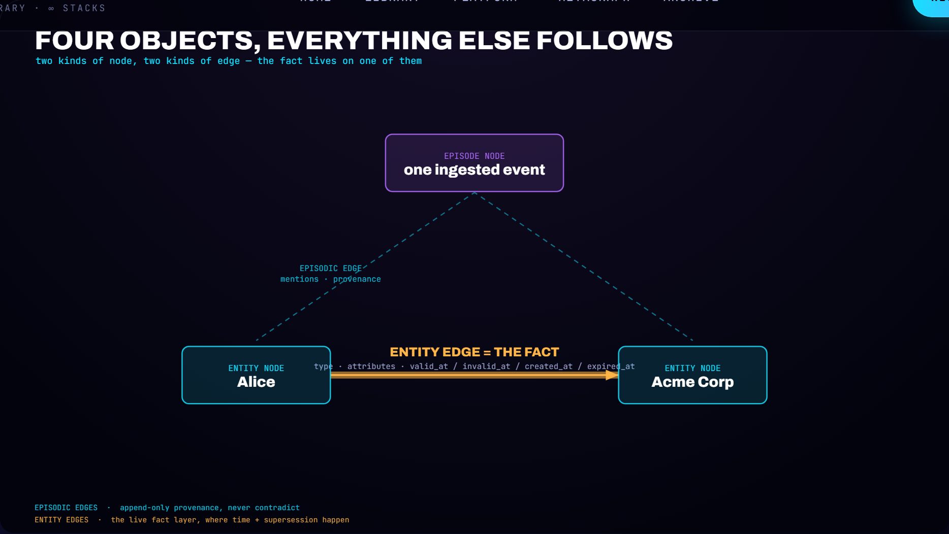
The two edge types get a separate figure because they fail in completely different ways. Episodic edges are append-only provenance; they grow without bound but they never contradict each other, because an episode either mentioned an entity or it didn't. Entity edges are the live fact layer, and they are where time, contradiction, and supersession all happen. When an answer is stale, it's an entity edge that went uninvalidated or unfiltered. When ingestion is expensive, it's the work of producing entity edges that costs. Keep the two clear in your head and you debug the right layer instead of chasing a ghost in the wrong one.
| Episodic edges | Entity edges | |
|---|---|---|
| What they are | Append-only provenance: this episode mentioned this entity. | The live fact layer, where time, contradiction and supersession all happen. |
| How they grow | Without bound, and they never contradict each other. | They open, close, and get superseded. |
| What goes wrong | Volume. | A stale answer is an entity edge that went uninvalidated or unfiltered. |
| Where the cost is | Storage. | Producing them, which is the work three LLM stages are doing. |
Four timestamps, not two
The phrase bi-temporal gets used loosely, so here's the concrete version. Every entity edge in Graphiti carries four timestamps, organized into two independent axes, and the whole correctness story depends on never collapsing them into one.
The first axis is valid time, which is about the world. valid_at is when the relationship became true in reality, and invalid_at is when it stopped being true. The second axis is system time, which is about the graph's own knowledge. created_at is when Graphiti learned the fact and wrote the edge, and expired_at is when Graphiti decided the fact was no longer current and closed it out. A person changing jobs in January that you only ingest in March produces an edge whose valid_at is January and whose created_at is March. The two-month gap between them is your system's epistemic lag: the time during which the graph was confidently wrong because it hadn't yet heard the news.
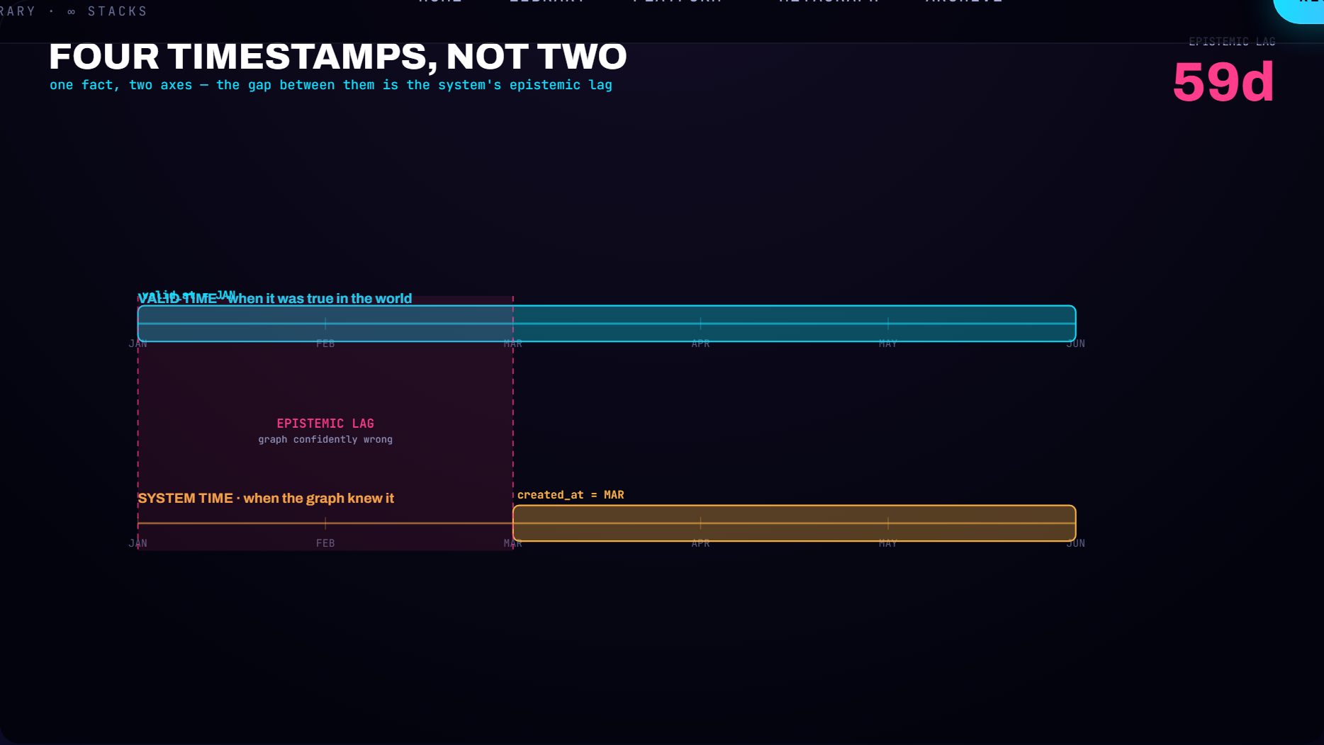
Holding both axes stops two different questions from colliding. What was true about this customer in February is a valid-time question, answered by filtering edges whose valid window contains February. What did the system believe about this customer when it sent that February email is a system-time question, answered by filtering on created_at and expired_at instead. Collapse the four timestamps into a single updated-at and both questions become unanswerable. The second one matters more than teams expect, because it's the question you ask when an agent made a bad decision and you need to know whether the data was wrong or the reasoning was. In practice valid_at and invalid_at are often inferred from the episode's reference time when the text gives no explicit date, which is reasonable, and it's also the first place silent error enters, because an inferred valid time is a guess stored as if it were a fact.
The ingestion pipeline, and where the money goes
Writing one episode into the graph runs a short pipeline, and three of its stages are LLM calls. That's the single most important operational fact about running Graphiti, because it tells you exactly where your latency and your bill come from. The stages run in order, and each one depends on the output of the one before it.
First the episode node is created, holding the raw content, its embedding, and its group and reference-time metadata. Then an LLM extracts the candidate entities from that text and classifies each into the entity types you defined. Then a second LLM call extracts the relationships among those entities, choosing an edge type for each pair your schema permits and pulling out the attributes that ride along, the start dates and roles and values. Then a third LLM step resolves each candidate entity against the entities already in the graph, deciding whether this Geoffrey Hinton is the one you already have or a new node. Only after all three model calls does the temporal materialization run, writing the episodic edges, writing or updating the entity edges, and applying the invalidation logic to anything the new facts supersede.
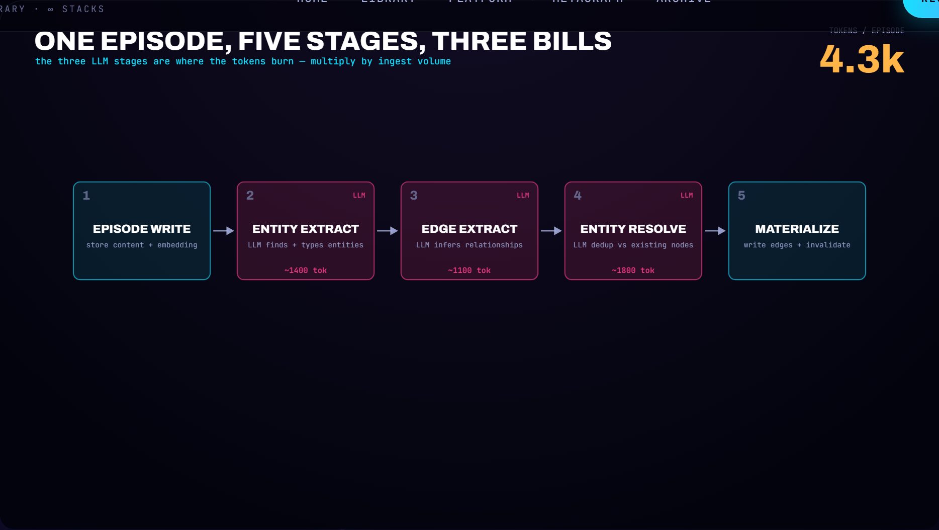
The shape of that pipeline dictates the shape of your cost. You pay model tokens per episode times the number of LLM stages, and you pay them again every time you reprocess. The mitigations Graphiti's authors arrived at are the ones the structure forces: batch episodes and parallelize the model calls while preserving per-episode chronology so supersession still happens in the right order, and constrain the ontology hard so the extractor is choosing among a small fixed set of entity and edge types rather than inventing structure. A tight ontology is a token-budget decision as much as a modeling preference, because every type you let the LLM invent is tokens spent describing it and noise spent cleaning it up later. Using smaller, cheaper models for the lighter stages is the direction of active work rather than a solved feature, so size your cost against current frontier-model pricing for the extraction and resolution calls and treat the cheaper path as a future improvement, not a present discount.
| Cost lever | What it does | What it costs you |
|---|---|---|
| Batch and parallelize the model calls | Runs the LLM stages across episodes at once. | Per-episode chronology has to be preserved anyway, so supersession still happens in the right order. |
| Constrain the ontology | The extractor chooses among a small fixed set of entity and edge types instead of inventing structure. | A tight ontology is a token-budget decision as much as a modeling preference. Every type you let the model invent is tokens spent describing it and noise spent cleaning it up later. |
| Smaller models on the lighter stages | The direction of active work. | Size your cost against current frontier-model pricing for extraction and resolution, and treat the cheaper path as a future improvement. |
| Reprocessing | Runs the same stages again over the same episodes. | You pay the model tokens again, every time. |
Entity resolution is the expensive heart
Of the three model stages, entity resolution is the one that decides whether your graph is worth anything, and it's also the one most likely to blow up your ingestion cost, because resolution is a per-candidate LLM decision. For each new entity the extractor proposes, Graphiti assembles a set of existing nodes it might be a duplicate of, sends that set plus the candidate to a model, and asks for a verdict: is this a duplicate, if so which existing node is it, and what is the merged summary. The model reasons over names and summaries to decide, which catches matches that string comparison misses and also costs strictly more.
The cost lives in the candidate set. You can't send every existing node as a comparison target, because that turns one ingestion into a scan of the whole graph, so the candidate set has to be pruned first to a small neighborhood by group, by entity type, and by embedding similarity before the model ever sees it. That pruning is itself work that needs the right indexes, and it is the lever that decides whether resolution costs you a bounded amount per entity or grows with the size of your graph. Get the pruning too broad and every ingestion drags in hundreds of comparison nodes and the bill scales with your data. Get it too narrow and you miss real duplicates, and the failure is the worse of the two.
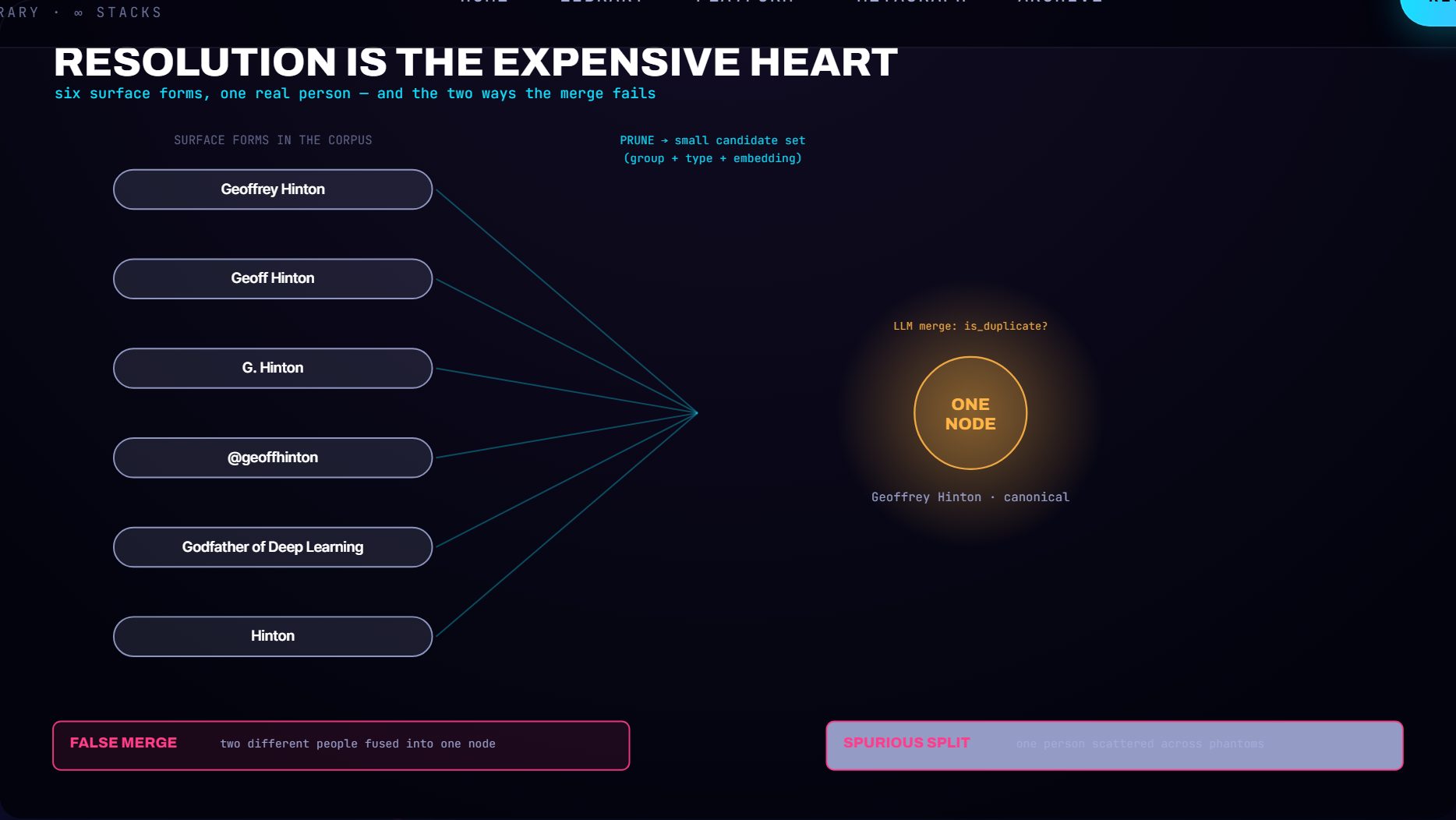
The two failure modes aren't symmetric, and they need different defenses. A false merge fuses two distinct entities into one node, and now every fact about either of them contaminates the other, and a contradiction engine downstream will see conflicts that are really just two people wearing one identity. A spurious split scatters one real entity across several phantom nodes. Now the facts that should have accumulated on one subject are spread thin across copies, real contradictions go undetected because the conflicting claims hang off different nodes, and a meta-claim disputing one copy is provenance attached to a fraction of the truth. The resolution step is the foundation the entire reified fact layer stands on, which is why it gets the most model budget and the most careful pruning, and why a year in production teaches you to watch its precision and recall the way you watch a load-bearing wall.
| Resolution failure | What it does to the graph | Why it needs its own defense |
|---|---|---|
| False merge | Fuses two distinct entities into one node, so every fact about either contaminates the other. | A contradiction engine downstream sees conflicts that are really two people wearing one identity. |
| Spurious split | Scatters one real entity across several phantom nodes, so facts that should have accumulated on one subject spread thin across copies. | Contradictions that genuinely exist go undetected, because the conflicting claims hang off different nodes, and a meta-claim disputing one copy attaches to a fraction of the truth. |
What invalidation does to an edge
When the world changes, Graphiti invalidates the old fact instead of deleting it. A new edge that contradicts or supersedes an existing one triggers the temporal logic to close the old edge's window, setting its invalid_at in valid time and its expired_at in system time to the moment the new fact takes over. Then the temporal logic writes the new edge open-ended until something supersedes it in turn. The old edge stays in the graph as history, removed from the current view but available to any query that asks about the past. Invalidation is the mechanism that makes time a first-class citizen instead of a column you overwrite, and it's also the mechanism that produced the stale-answer failure at the top of this essay, because it only protects you if your queries honor it.
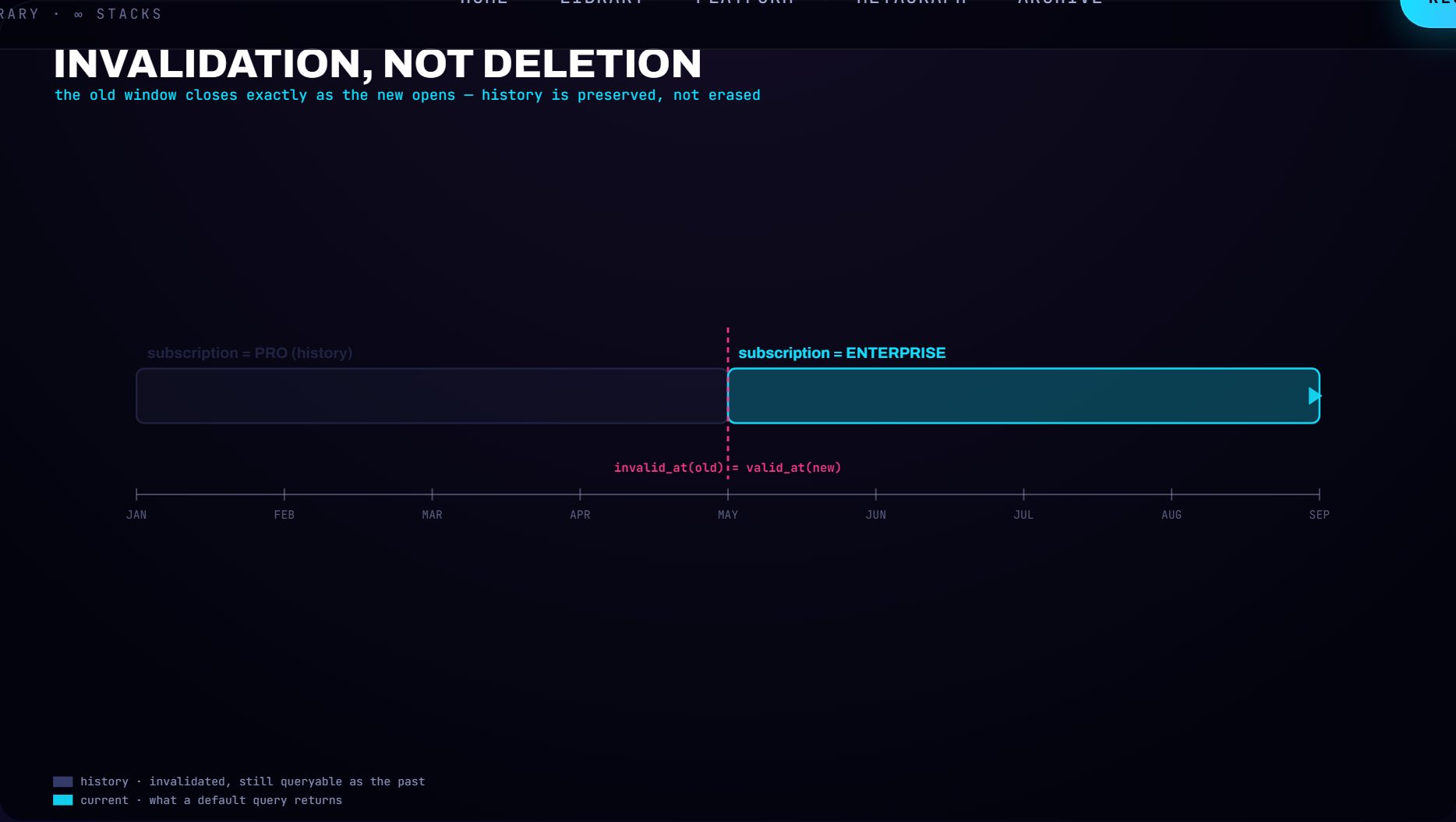
The decision that nobody configures explicitly, and the one that bites hardest, is which relationships are single-valued and which are multi-valued. A single-valued relationship is a state: a person has one current employer, an account has one current subscription tier, an entity has one canonical name. When a new fact arrives on a single-valued edge, it is a state change, and the old edge must be invalidated. A multi-valued relationship is additive: a person has many interests, a company has many partners, and a new fact there joins the old ones instead of contradicting them. Graphiti's temporal logic leans on this distinction to decide what supersedes what, and the exact rules for what counts as the same dimension are more design-intent than published specification. So the safe production posture is to treat single-valued versus multi-valued as a schema decision you make deliberately per edge type, not a behavior you assume the framework infers correctly for you. Encode it where you control it, because discovering after six months that the graph treated employer as additive and accumulated five simultaneous current jobs per person is the kind of error that's cheap to prevent and expensive to unwind.
The queries that destroy clusters
Underneath Graphiti is a property graph, and a property graph has a small number of query shapes that go from instant to ruinous as the data grows. None of them show themselves at demo scale, and all of them are waiting at ten million edges. The first and worst is the supernode.
A supernode is a node with very high degree: the popular customer with a hundred thousand episodes, the product referenced in millions of facts, the low-cardinality status node that a million items all point at. It hurts for a structural reason, and the fix follows from the cause. When a query reaches a node and expands its relationships, the cost of that expansion is proportional to the node's degree. There's no index that lets the engine consider three of a million edges and skip the rest; the adjacency list is the only structure at that step, and traversal is pointer-chasing down it. A variable-length pattern that passes through a supernode fans out to its entire neighborhood at every hop, the planner's cardinality estimates go wildly wrong, and a query that returned in milliseconds against a test graph spends minutes against production and pulls the whole cluster's latency down with it.
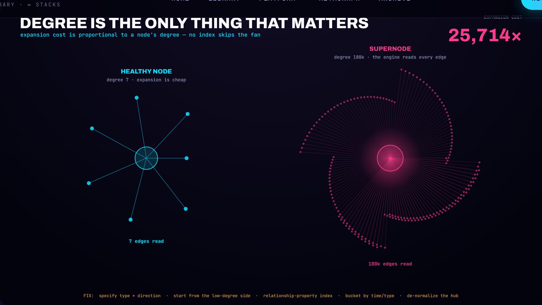
The defenses are concrete because the cause is. Always specify relationship type and direction in the pattern, so the engine filters to the right slice of the adjacency list instead of scanning every edge in both directions. Start the traversal from the low-degree side, seeding on a selective node index and expanding toward the supernode rather than from it, so the dense node is never the starting expansion point. Put a property index on the relationship and constrain on it, so a selective filter like a time window can become a relationship-index scan instead of a full fan. Bucket by time or type, so a node's millions of edges route through intermediate bucket nodes and a query for one window touches one bucket. And refactor the worst offenders out of existence: a low-cardinality hub like a status node is better expressed as an indexed property on the items than as a node a million edges point at. Every one of these reduces the degree that any single expansion has to pay for, which is the only quantity that matters.
| Defense against a supernode | What it changes |
|---|---|
| Specify relationship type and direction in the pattern | The engine filters to the right slice of the adjacency list instead of scanning every edge in both directions. |
| Start from the low-degree side | Seed on a selective node index and expand toward the dense node, so it is never the starting expansion point. |
| Put a property index on the relationship and constrain on it | A selective filter such as a time window becomes a relationship-index scan instead of a full fan. |
| Bucket by time or type | A node's millions of edges route through intermediate bucket nodes, so a query for one window touches one bucket. |
| Refactor the worst offenders away | A low-cardinality hub such as a status node becomes an indexed property on the items instead of a node a million edges point at. |
The second expensive shape is the point-in-time query itself, and it carries a trap that surprises people who assume a composite index will save them. A validity filter, valid_at <= T AND invalid_at > T, is an interval-contains-point question, and a property graph has no native interval index for it. There's no equivalent of a spatial range index that understands the pair as an interval. What you get from a range index on one bound is a one-dimensional seek that narrows the candidates, after which the other bound is applied as an ordinary filter over whatever the seek returned. A composite index on both bounds doesn't rescue the query, because it orders by the leading key and then filters, rather than treating the two together as an interval the index can probe.
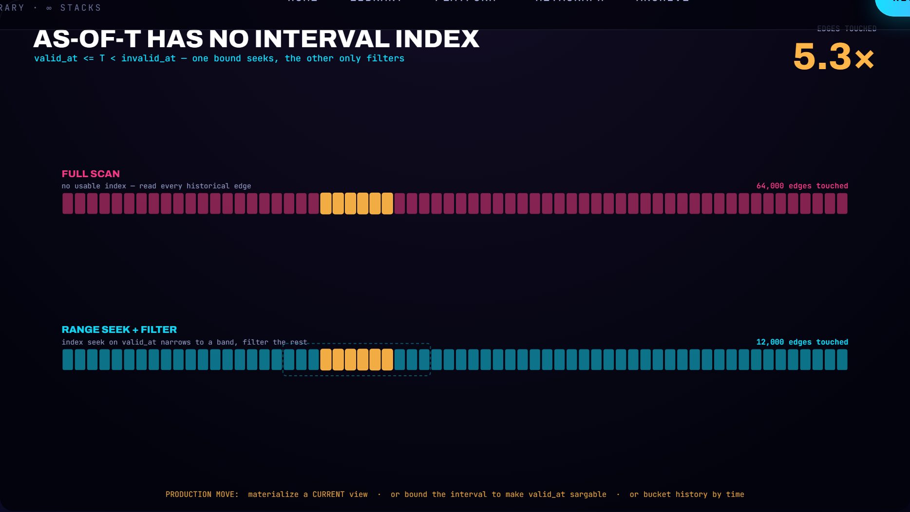
So the production patterns work around the missing index rather than wishing for it. The most common query is as-of-now, and the cleanest answer to it is to materialize a current view: keep currently-valid edges plain and open-ended, and move expired edges to a history label or a separate relationship type, so the everyday query never touches the historical mass and never evaluates an interval at all. When you do need as-of-some-past-time, add a maximum-interval-duration bound if your domain has one, turning an open-ended leading bound into a sargable range the index can seek. And bucket history by time the same way you bucket a supernode, so an as-of query for one month reads one month's edges. The interval index you want doesn't exist in this world; the structure that replaces it is the current-versus-history split, and building it before you have ten million historical edges is far cheaper than retrofitting it after.
Hybrid search and the user at the center
Graphiti's search combines three signals: vector similarity over embeddings, BM25 full-text over the lexical content, and graph traversal that reranks candidates by their distance from a central node, usually the user or account the query is about. The first two find things that are semantically and lexically relevant; the third pulls the relevant-in-general down in favor of the relevant-to-this-subject, which is the move that makes the answer feel like memory rather than search.
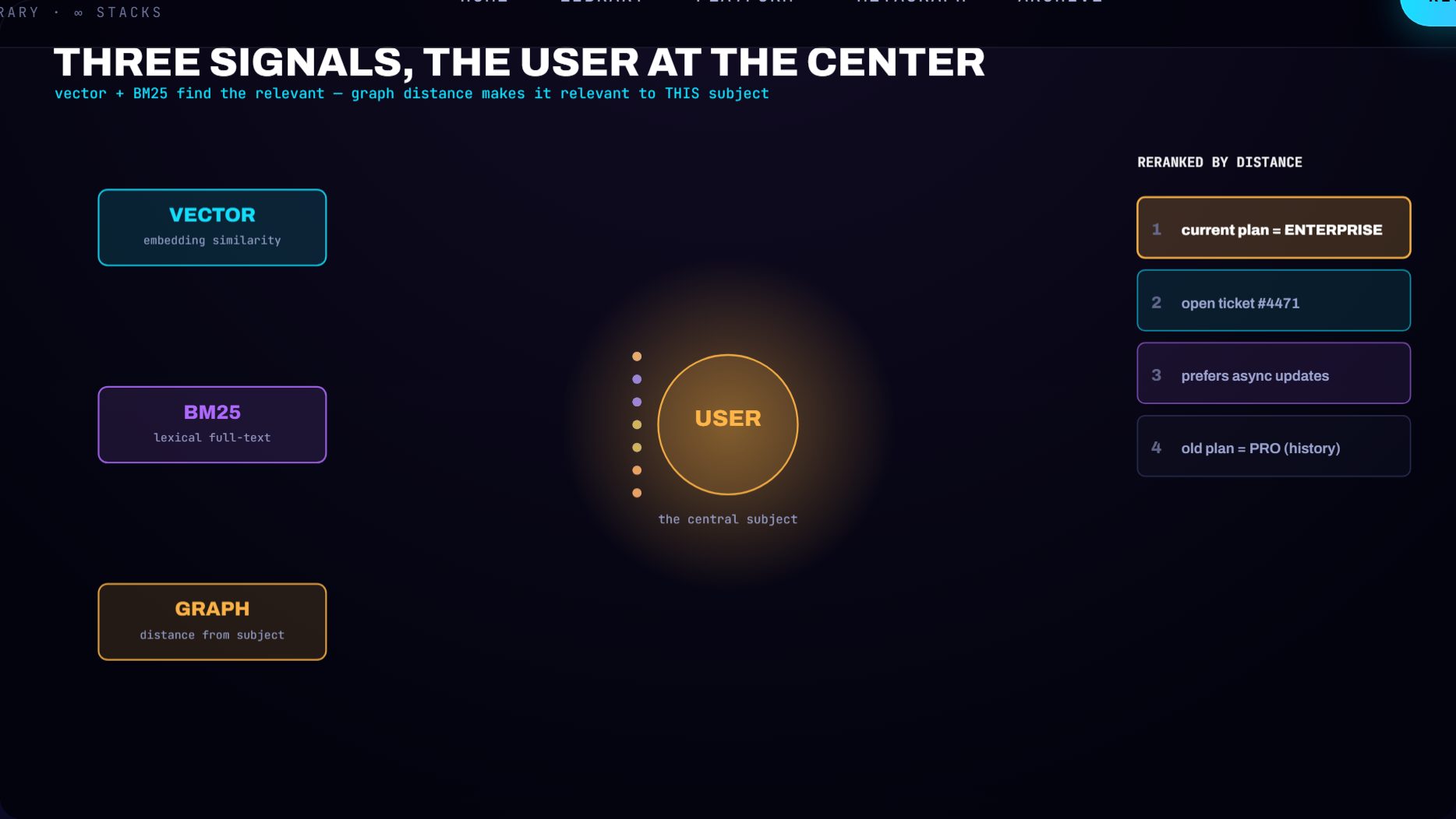
The operational catch is that all three signals have to be fed and tuned together, and the graph-distance leg is where the supernode problem returns. Reranking by distance means traversal, traversal near a central node means expanding that node's neighborhood, and a central node that is a heavy user is a supernode by another name. The same discipline applies: cap the depth, lean on hybrid search to fetch a small candidate neighborhood first and traverse locally inside it rather than walking the global graph, and keep embedding strategies for episodes and entities aligned so the vector leg is comparing like with like. Done right, distance reranking is the feature that justifies the whole temporal graph over a plain vector store, because a customer whose situation changed last week is served the current state with the old state correctly demoted. Vector-only retrieval can't do that, because it has no notion that one of two similar facts has been superseded.
The schema decisions you cannot take back
The hardest lessons are the ones that arrive as documentation footnotes and land as migration projects. Graphiti documents plainly that several core schema choices are only reversible by re-ingesting your data into a fresh graph, which means they aren't really reversible at all once your source episodes are large or no longer fully retained. Three of them deserve to be understood before you write your first episode.
Entity type design is the first. You can add new entity types for future episodes freely, but existing nodes stay untyped, and giving old data the benefit of a new type means re-ingesting it into a new graph. Over-generalize early, make everything a generic entity, and your first months of data lack the structured attributes and the type discrimination that everything downstream relies on, and you can't retrofit that structure without reprocessing. Edge naming is the second, and it carries a subtlety that's easy to miss: a custom edge type is stored in the edge's name field, and that field is the type everywhere in the system. Renaming or splitting an edge type later is a data migration across every edge of that name plus the query logic that keyed on it. And the edge-type map, the schema of which relationships are even allowed between which entity-type pairs, shapes what the extractor can produce; start it too loose and your early graph fills with generic relate-to edges that resist retrofitting into anything specific.
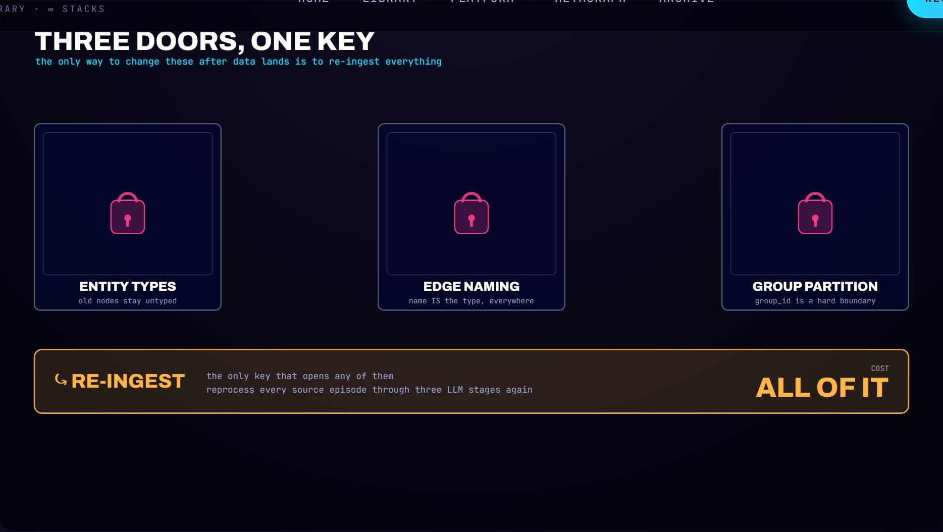
The third is group_id, the namespace key on every node and edge, and it's a hard partition by design. Same group means one isolated graph; different groups never traverse into each other, and a cross-tenant or cross-domain view is something you assemble in your application by querying several groups and merging, not something the graph does for you. Choose the partitioning early, per user or per tenant or per domain, and changing it later means migrating data into a new scheme. The guidance cuts both ways: too many namespaces fragments your data into pieces too small to be useful, too few sacrifices the isolation and the per-graph performance that keeping graphs small and local buys you. Partitioning is also the lever that quietly solves the supernode and the interval-scan problems at the same time, because a graph kept small by deliberate partitioning has fewer dense nodes and shorter history to scan. That makes the partitioning decision a performance decision that looks like a multi-tenancy one.
What a year actually teaches
The lessons compound into a short list of postures, each one the residue of a specific failure. Constrain the ontology before you ingest, because every entity and edge type you leave open is tokens at extraction and noise at query, and a tight schema is the cheapest lever on both cost and quality. Decide single-valued versus multi-valued per edge type on purpose, so state changes invalidate and additive facts accumulate, instead of discovering the framework guessed wrong after a person has five current employers. Index the temporal fields and build the current-versus-history split before you have the history, because the interval index you'll wish for doesn't exist and the materialized current view is the structure that replaces it. Partition with group_id deliberately, because it's simultaneously your tenancy boundary and your defense against supernodes and long historical scans. And write every retrieval to honor invalidation, because the stale answer at the top of this essay came from a query that filtered on type and forgot to filter on time.
What's solidly proven is the core: episodes, entities, the two edge types, the four-timestamp bi-temporal model, invalidation rather than deletion, LLM-driven extraction and resolution, group-based namespacing, and hybrid search with distance reranking. These run in Zep's hosted product and in adopters' deployments, and the schema-stickiness lessons are documented from real users who had to re-ingest. What remains closer to design intent than to published proof is the behavior at the very top of the scale (the latency distributions and supernode dynamics on multi-billion-edge graphs) and the exact internal rules that decide when one fact supersedes another. The property-graph behaviors underneath, the supernode cost and the missing interval index, come from how Neo4j and FalkorDB plan queries, so they hold for whatever you build on those engines. A year with the system is mostly a year of learning that the temporal model gives you the right shape for free and asks you to do the unglamorous work of querying it correctly, partitioning it deliberately, and deciding its schema before the data makes the decision permanent for you.
| Solidly proven, running in Zep's hosted product and in adopters' deployments | Closer to design intent than to published proof |
|---|---|
| Episodes, entities, and the two edge types | Behaviour at the very top of the scale: latency distributions and supernode dynamics on multi-billion-edge graphs |
| The four-timestamp bi-temporal model | The exact internal rules that decide when one fact supersedes another |
| Invalidation rather than deletion | |
| LLM-driven extraction and resolution | |
| Group-based namespacing | |
| Hybrid search with distance reranking | |
| The schema-stickiness lessons, documented from real users who had to re-ingest | |
| The property-graph behaviours underneath: supernode cost and the missing interval index, which follow from how Neo4j and FalkorDB plan queries |
The next essay turns to the system Graphiti is most often weighed against on the correctness axis, OpenCog Hyperon, and gives it the same treatment: what the AtomSpace delivers, where the cognitive architecture is research-grade rather than production-ready, and how to read the gap between the two without the marketing in the way.
END OF ESSAY 08 · CONTINUE TO ESSAY 09 →